Thursday, July 31, 2008

Escaping transcendence

When I was a teenager I was fond of 19th century novels such as Flaubert's Sentimental Education or Dostoevsky's Crime and Punishment. In music, my absolute favorite were Pink Floyd's long, discursive compositions: I remember myself those days listening to Comfortably Numb over and over again full of adolescent angst.

There was a uniting theme to these works: they were important, no pastime, bigger than life in some sense. The subjects proposed were deliberately profound: morality, redemption, isolation. There was a search for some sort of transcendence in the literature and music I visited in my youth days.

Twenty years later, I found myself reading Pynchon's Gravity's Rainbow and appreciating the beauty of Portishead's new album, Third. The contrast is stark: some profundity remains, but in a subtler form. Discourse has been supplanted by evocation, and layers of reference take the place of the distinctive stories of the past. Whereas the pieces of my youth sought to prove some thesis or convey important information to a more or less passive audience, Rainbow or Third draw heavily from the reader/listener mental background and cannot exist in isolation from the audience and their implied cultural setting.

I think this is a recurring pattern in the way art has evolved in our days: we have moved from transcendence to self-reference. Art today is less about the world and much more about art itself and its relationship with the viewer. If artistic works of the past projected the viewer into a bigger, external reality, current art constitutes a mere tool for exquisite masturbation.

Sunday, July 27, 2008

Indirect survey

The usual way to statistically determine the prevalence of a given trait T in a population involves selecting a representative population sample and having their members answer the question "Do you have trait T?"; the number of affirmative questions divided by the size of the sample is an estimate of the actual prevalence of p = P(T). How can we estimate p if the following question is used instead?

Do you have some friend with trait T?

Let us assume that having a friend with T is independent of the fact that other friends may or may not have T. The probability then that a person has a friend with T is given by:

p' = 1 − ∑fi(1 − p)i,
fi := P(a person has exactly i friends).

So, p' is simply 1 − GF(1 − p), where GF is the probability-generating function of F, the random variable expressing the number of friends a person has. If we model F by a Poisson distribution with mean λ, we have

GF(x)= eλ(x − 1)

and

p' = 1 − eλp,
p = −(1/λ) ln(1 − p').

The figure shows p' as a function of p for various values of λ.

There are situations where it can be interesting to estimate p through this indirect survey method:

  1. For usual values of λ much greater than 1 , p' is notably larger than p when the latter lies in the vicinity of 0. This implies that indirect estimation of p through p' results in better (narrower) confidence intervals when p is very small. For instance, for p = 1/1000 and λ = 10 a direct survey obtains on average one affirmative answer in a sample of 1000 individuals, with an associated 95% Wilson score confidence interval of (0.0001, 0.0065) (calculated via VassarStats). With an indirect survey we typically get 10 affirmative answers for the same size of population, with a confidence interval (0.0051, 0.019) associated to p'; applying the transformation p = −(1/λ)ln(1 − p'), the latter confidence interval maps to (0.0005, 0.0019), whose width is ~20% of that of the interval for the direct survey.
  2. When doing surveys on sensitive issues (illegal drug use, paid sex usage) results can be severely biased due to the reluctance of people to answer thruthfully. In these cases, survey respondents might be more inclined to answer accurately when the questions are indirect: it is easier for a person to recognize that he has friends who had paid for sex than admitting paying for sex oneself.

A serious drawback of this method is its reliance on the a priori unkown parameter λ. One technique for solving this is the following: include into the survey an additional control question for which the associated statistics are already known, so that the survey results can be used to estimate λ. Ideally, the control question's subject matter should be similar to that of the actual question so as to cancel evasive answer bias out.

Wednesday, July 23, 2008

Formalizing predicate boundedness

Informally, we defined a predicate F to be bounded if the entities for which F is true can be enclosed in a reasonably "small" class. Of course, for this definition to be of any use we have to clearly specify what we mean by "small", or at least use our intuition to propose some axioms for this concept:

  • If A and B are small, A U B is small.
  • If A and B are small, AB is small.
  • If A is small and B is included in A, B is small.
  • If A is small then −A, the class of all entities outside A, is not small.

In the definition of −A given above we have assumed that we are working inside some universal class comprising any conceivable entity.

The axioms for "small" are far from categorical. We give a few models for this notion:

  • If we decide to work within a mathematical class theory such as NBG, there is an easy definition for "small": A class is small if it is a set (not all classes are sets).
  • We can take "small" as meaning "finite", provided the universal class is infinite, or as having cardinality less than or equal to some fixed infinite cardinal κ, provided the universal class is larger than κ.
  • Suppose we have a fixed set of "primitive" predicates Fi with domains Di such that UDi is smaller than the universal class. We can define the class of small sets as the least class S comprising all Di that is closed under finite union, finite intersection and comprehension: if X belongs to S and Y is a subset of X, Y belongs to S. This definition of "small" can be seen as a formal model for Quine's notion of natural kinds.

This is probably as far as we can get with respect to defining what "small" means in the context of predicate boundedness.

Saturday, July 19, 2008

Cpp bignum arithmetic: part II

After having studied addition, subtraction and multiplication of C preprocessor bignums, let us now turn to division. To gain some insight into the mechanics of the division algorithm we reproduce a division layout the way we were taught to do at school:

‎         20553
‎8879265 |432
‎ 239
‎ 2392
‎ 2326
‎ 1665
‎ 369

To divide 8879265 by 432, we begin by isolating the first 3-digit group of the dividend, 887, and calculate how many times the divisor 432 makes it into it; we have that 887 = 432·2 + 23, so 2 is the first digit of our result, and we write down the remainder 23. Next, we append the next digit of the dividend, 9 , to the remainder and proceed iteratively:

  • 887 = 432·2 + 23,
  • 239 = 432·0 + 239,
  • 2392 = 432·5 + 232,
  • 2326 = 432·5 + 166,
  • 1665 = 432·3 + 369

Let us assume we have a macro BN_QDIGIT_REMAINDER(bn1,bn2) that returns a sequence (q)(r), where q is the greatest digit between 0 and 9 such that bn2·qbn1 and r is the bignum representing the value bn1bn2·q. We can then implement the division of bn1 = (bn11)···(b1n) by bn2 (bn21)···(b2m)by folding over reverse((bn1m)···(b1n)) with the following recursive state definition:

statei = (leadi,bn2,resi);
state
0 = ((bn11)···(b1m-1), bn2,empty sequence),
leadi+1 = first(BN_QDIGIT_REMAINDER(leadi,bn2)),
resi+1 = append(resi, second(BN_QDIGIT_REMAINDER(leadi,bn2))),

where the functions first and second simply return the first and second component of a sequence of size 2. This is the complete Boost.Preprocessor-based algorithm:

‎#define BN_DIV(bn1,bn2) \
‎BOOST_PP_IF( \
‎ BN_LESS(bn1,bn2), \
‎ BN_DIV_CASE1, \
‎ BN_DIV_CASE2)(bn1,bn2)

‎#define BN_DIV_CASE1(bn1,bn2) (0)

‎#define BN_DIV_CASE2(bn1,bn2) \
‎BN_DIV_POSTPROCESS( \
‎ BOOST_PP_SEQ_TAIL(BN_DIV_STATE_RESULT(\
‎ BOOST_PP_SEQ_FOLD_LEFT( \
‎ BN_DIV_OP, \
‎ ( \
‎ (0) \
‎ BOOST_PP_SEQ_FIRST_N( \
‎ BOOST_PP_DEC(BOOST_PP_SEQ_SIZE(bn2)),bn1)) \
‎ (bn2) \
‎ ((~)), \
‎ BOOST_PP_SEQ_REST_N( \
‎ BOOST_PP_DEC(BOOST_PP_SEQ_SIZE(bn2)),bn1)))))

‎#define BN_DIV_POSTPROCESS(result) \
‎BOOST_PP_IF( \
‎ BOOST_PP_EQUAL(0,BOOST_PP_SEQ_ELEM(0,result)), \
‎ BOOST_PP_SEQ_TAIL, \
‎ BN_DIV_POSTPROCESS_CASE2)(result)

‎#define BN_DIV_POSTPROCESS_CASE2(result) result

‎#define BN_DIV_OP(s,state,x) \
‎BN_DIV_OP_IMPL( \
‎ BN_QDIGIT_REMAINDER( \
‎ BN_DIV_STATE_LEAD(state)(x), \
‎ BN_DIV_STATE_BN2(state)), \
‎ BN_DIV_STATE_BN2(state), \
‎ BN_DIV_STATE_RESULT(state))

‎#define BN_DIV_OP_IMPL(qr,bn2,result) \
‎(BOOST_PP_SEQ_ELEM(1,qr)) \
‎(bn2) \
‎(result(BOOST_PP_SEQ_ELEM(0,qr)))

‎#define BN_DIV_STATE_LEAD(state) BOOST_PP_SEQ_ELEM(0,state)
‎#define BN_DIV_STATE_BN2(state) BOOST_PP_SEQ_ELEM(1,state)
‎#define BN_DIV_STATE_RESULT(state) BOOST_PP_SEQ_ELEM(2,state)

We are then left with the task of implementing the macro BN_QDIGIT_REMAINDER(bn1,bn2). A brute-force approach is to try the digits 9,8,...,0 until we met the first one satisfying bn2·qbn1, but this is unnecesarily wasteful: we find in Brinch Hansen's paper "Multiple-length division revisited" the following nice theorem: if bn1 and bn2 are represented in such a way that length(bn1) = length(bn2) +1 (even if that means bn1 has to be padded with some some leading zeros) and we define

qe =min(9, floor((bn11·100 + bn12·10 + bn13)/(bn21·10 + bn22))),

then

qqeq + 1,

that is, we can use the first three digits of bn1 and the first two digits of bn2 to estimate q and will be off at most by one:

‎#define BN_QDIGIT_REMAINDER(bn1,bn2) \
‎BN_QDIGIT_REMAINDER_IMPL( \
‎ BN_ZERO_SEQ( \
‎ BOOST_PP_IF( \
‎ BOOST_PP_LESS_EQUAL( \
‎ BOOST_PP_SEQ_SIZE(bn1), \
‎ BOOST_PP_SEQ_SIZE(bn2)), \
‎ BOOST_PP_INC( \
‎ BOOST_PP_SUB( \
‎ BOOST_PP_SEQ_SIZE(bn2), \
‎ BOOST_PP_SEQ_SIZE(bn1))), \
‎ 0))bn1, \
‎ bn2)

‎#define BN_ZERO_SEQ(n) \
‎BOOST_PP_REPEAT(n,BN_ZERO_SEQ_OP,~)

‎#define BN_ZERO_SEQ_OP(z,n,data) (0)

‎#define BN_QDIGIT_REMAINDER_IMPL(bn1,bn2) \
‎BOOST_PP_IF( \
‎ BOOST_PP_LESS(BOOST_PP_SEQ_SIZE(bn2),2), \
‎ BN_QDIGIT_REMAINDER_CASE1, \
‎ BN_QDIGIT_REMAINDER_CASE2)(bn1,bn2)

‎#define BN_QDIGIT_REMAINDER_CASE1(bn1,bn2) \
‎BN_QDIGIT_REMAINDER_CASE1_RETURN( \
‎ BOOST_PP_ADD( \
‎ BOOST_PP_MUL(BOOST_PP_SEQ_ELEM(0,bn1),10), \
‎ BOOST_PP_SEQ_ELEM(1,bn1)), \
‎ BOOST_PP_SEQ_ELEM(0,bn2))

‎#define BN_QDIGIT_REMAINDER_CASE1_RETURN(n1,n2) \
‎(BOOST_PP_DIV(n1,n2))((BOOST_PP_MOD(n1,n2)))

‎#define BN_QDIGIT_REMAINDER_CASE2(bn1,bn2) \
‎BN_QDIGIT_REMAINDER_CASE2_TEST( \
‎ bn1,bn2, \
‎ BN_DIV_RRR_DD( \
‎ BOOST_PP_ADD( \
‎ BOOST_PP_MUL(BOOST_PP_SEQ_ELEM(0,bn1),10), \
‎ BOOST_PP_SEQ_ELEM(1,bn1)), \
‎ BOOST_PP_SEQ_ELEM(2,bn1), \
‎ BOOST_PP_SEQ_ELEM(0,bn2), \
‎ BOOST_PP_SEQ_ELEM(1,bn2)))

‎#define BN_QDIGIT_REMAINDER_CASE2_TEST(bn1,bn2,q) \
‎BN_QDIGIT_REMAINDER_CASE2_TEST_IMPL(bn1,bn2,q,BN_DIGIT_MUL(bn2,q))

‎#define BN_QDIGIT_REMAINDER_CASE2_TEST_IMPL(bn1,bn2,q,bn2q) \
‎BOOST_PP_IF( \
‎ BN_LESS_WITH_ZERO(bn1,bn2q), \
‎ BN_QDIGIT_REMAINDER_CASE2_TEST_IMPL_CASE1, \
‎ BN_QDIGIT_REMAINDER_CASE2_TEST_IMPL_CASE2)(bn1,bn2,q,bn2q)

‎#define BN_QDIGIT_REMAINDER_CASE2_TEST_IMPL_CASE1(bn1,bn2,q,bn2q) \
‎(BOOST_PP_DEC(q))(BN_SUB(bn1,BN_SUB(bn2q,bn2)))

‎#define BN_QDIGIT_REMAINDER_CASE2_TEST_IMPL_CASE2(bn1,bn2,q,bn2q) \
‎(q)(BN_SUB(bn1,bn2q))

‎#define BN_LESS_WITH_ZERO(bn1,bn2) \
‎BOOST_PP_IF( \
‎ BOOST_PP_EQUAL(BOOST_PP_SEQ_ELEM(0,bn1),0), \
‎ BN_LESS_WITH_ZERO_CASE1, \
‎ BN_LESS)(bn1,bn2)

‎#define BN_LESS_WITH_ZERO_CASE1(bn1,bn2) \
‎BN_LESS(BOOST_PP_SEQ_TAIL(bn1),bn2)

The code above invokes the macro BN_DIV_RRR_DD(r1r2,r3,d1,d2) whose behavior is defined by:

BN_DIV_RRR_DD(r1r2,r3,d1,d2) = floor((r1r2·10 + r3)/(d1·10 + d2)).

The operation cannot be done directly because Boost.Preprocessor-based arithmetics are limited to numbers between 0 and BOOST_PP_LIMIT_MAG = 256. Instead, floor(r1r2/d1) is used as an initial upper-bound estimation which is then adjusted to the correct value using arithmetic operations that never exceed the BOOST_PP_LIMIT_MAG limit. The implementation of BN_DIV_RRR_DD is somewhat cumbersome but conceptually simple.

The complete implementation of all four arithmetic operations --addition, subtraction, multiplication and division-- is provided. Cpp bignum arithmetic is not very fast; for instance, given the following calculation of 30!:

‎BN_TO_LITERAL(
‎ BN_MUL((3)(0),BN_MUL((2)(9),BN_MUL((2)(8),BN_MUL((2)(7),
‎ BN_MUL((2)(6),BN_MUL((2)(5),BN_MUL((2)(4),BN_MUL((2)(3),
‎ BN_MUL((2)(2),BN_MUL((2)(1),BN_MUL((2)(0),BN_MUL((1)(9),
‎ BN_MUL((1)(8),BN_MUL((1)(7),BN_MUL((1)(6),BN_MUL((1)(5),
‎ BN_MUL((1)(4),BN_MUL((1)(3),BN_MUL((1)(2),BN_MUL((1)(1),
‎ BN_MUL((1)(0),BN_MUL((9) ,BN_MUL((8) ,BN_MUL((7),
‎ BN_MUL((6) ,BN_MUL((5) ,BN_MUL((4) ,BN_MUL((3),
‎ (2))))))))))))))))))))))))))))))

it takes around 20 seconds for this expression to expand to

265252859812191058636308480000000

using GCC 3.4.4 for Cygwin in a Windows box with a 1.66 GHz Intel Core 2 Duo and 1 GB RAM. Within the same environment, the long division

‎BN_TO_LITERAL(
‎ BN_DIV(
‎ (2)(6)(5)(2)(5)(2)(8)(5)(9)(8)(1)(2)(1)(9)(1)(0)(5)
‎ (8)(6)(3)(6)(3)(0)(8)(4)(8)(0)(0)(0)(0)(0)(0)(0),
‎ (1)(8)(3)(7)(0)(8)(0)(0)))

takes around 12 seconds. In a later entry, we will explore ways to improve the performance of bignum multiplication and division through memoization techniques.

Tuesday, July 15, 2008

1015 + 6 = 1000000000000005.9

In a prior entry we saw how the internal representation of numbers in Google Docs spreadsheets as double precision IEEE 754 floating point quantities introduces rounding errors when the stored values get larger than 253. Yet, this does not explain the fact that 19! is displayed as 121645100408831984, since 19!=121645100408832000 can be represented exactly in double precision IEEE 754.

Let us see how numbers are rounded in the vicinity of 121645100408832000:

Each number on the left column is the least value that gets rounded off to the associated number on the right column: for instance, the numbers 1216···1945 ≤ n ≤ 1216···1959 get mapped to 1216···1952, and so on. Except for the rows in bold, each rounding interval is comprised of 17 or 15 numbers (instead of each interval being of length 16, due to the application of unbiased rounding) around its central value. This is entirely reasonable because 19! is 57 bits wide and double precision IEEE 754 can only represent up to 53 significant bits, hence the hops of size 257−53 = 16. On the other hand, we have an anomaly between rows 4 and 5: the values from 1216···1992 to 1216···2008, which should map to 1216···2000, are instead rounded off to the preceding value 1216···1984.

The binary representation of 19! has 57 bits: if we divide by 16 we get the 53 bit wide number 7602818775552000, which ought be exactly representable in double precision IEEE 754. Pasting this into a Google Docs spreadsheet gets us:

which is off by one! If we keep dropping least significant bits from this number (i.e. dividing by 2) we obtain this:

Only the last number is shown correctly, but after that the display is correct all the way down to zero. This suggests that there is a lower limit below which we do not have displaying problems. After probing the number space more or less thoroughly, our findings are the following:

The problems occur from 1015 up. Displaying errors are extremely frequent and distributed very evenly: if we consider the sequence of exactly representable integers greater than 1015, roughly 11% of them are displayed incorrectly, with a typical distance between consecutive errors of 9, ocasionally a little more. The magnitud of the error is ~n/253. The smallest number displayed incorrectly is 1015 + 6 = 1000000000000006, which Google Docs spreadsheets show as 1000000000000005.9.

The problem seems to be related only to the displaying algorithm; numbers are stored correctly, as suggested by the following:

Friday, July 11, 2008

Hempel's paradox and bounded predicates

If a naturalist decides to inductively prove the sentence

All ravens are black

she is expected to go out to the country and seek for ravens, checking the color of every raven sighted. After numerous individual confirmations the naturalist feels confident to inductively generalize and declare the sentence "all ravens are black" true. But this sentence is logically equivalent to

Everything that is not black is not a raven.

Now, to obtain confirmation of this sentence the naturalist need not even leave home! All she has to do is look for things around the room which are not black and check out that they are not ravens. There is a myriad of valid instances outside the realm of ornitology, so it seems one can take the inductive step without even having sighted a single raven.

One of the most usual resolutions of Hempel's Paradox follows a statistical or Bayesian approach: sighting a black raven provides evidence that all ravens are black in a much higher degree than sighting a non-black thing which is not a raven (vg. a green apple) because there are many fewer ravens than non-black things. Without going into discussing this argument, I would like to point out that the observation "there are fewer ravens than non-black things" can be interpreted in an ontological sense that is far stronger than the mere fact that the cardinal of the set of ravens is less than the cardinal of the set of non-black things. Furthemore, I contend that it is this ontological interpretation that gives Hempel's puzzle its paradoxical flavor.

Consider the formulation of "all ravens are black" in first order logic:

for all x (RxBx),

where R is the predicate for "raven" and B for "black". This sentence is equivalent to:

for all x (−Bx → −Rx),

as we already knew. Both formulations are instances of the general schema:

for all x (ΦxΨx)

where Φ = R in the first case and Φ = −B in the second case. This first order logic formulation is not explicit about the universe of discourse considered, that is, the class U of entities over which x is meant to range. It is naturally expected that U is large enough that it contains all the objects for which Φ is true, while being small enough so that the elements considered are relevant to the sentence. So, for the case Φ = R the following are natural universes of discourse:

  • The class of all corvids
  • The class of all birds
  • The class of all macroscopic animals

Now, what is a natural universe of discourse for the formulation in which Φ = −B? The chosen class U must contain all things non-black, but not being black is a property held by ontologically remote entities:

  • Kingfishers are not black
  • Daffodils are not black
  • Rubies are not black
  • Quarks are not black
  • Emotions are not black
  • π is not black
  • Sets are not black

It seems that, short of taking U to be the class of everything, we cannot choose a universe of discourse comprehensive enough: almost anything is not black.

And this is, in my opinion, the ontological qualm behind Hempel's paradox: When applying induction to prove "for all x (ΦxΨx)" we expect that Φ is a bounded predicate, i.e. one for which a natural universe of discourse exists. "Raven" is a bounded predicate, whereas "non-black" is not. The Bayesian explanation of the paradox assumes that a universe of discussion has already been established, but it is the very choice of universe that poses the problem.

In a later entry we will try to give some formalization to the notion of a predicate being bounded using some elementary set theory machinery.

Monday, July 7, 2008

Cpp bignum arithmetic: part I

Adding two C preprocessor bignums is an easy task, we have to merely reproduce the basic algorithm taught at elementary school; if the bignums to add are bn1 and bn2 and length(bn1) ≥ length(bn2) (otherwise we just swap them), we can fold over reverse(bn1), similarly as how we did for bignum comparison, using the following recursive state definition:

statei = (carryi,seqi,resi);
state
0 = (0, reverse(bn2),empty sequence),
carryi+1 = addmsd(reverse(bn1)i,head(seqi),carryi),
seqi+1 = tail(seqi),
resi+1 = append(resi, sublsd(reverse(bn1)i,head(seqi),carryi)),

where addmsd and addlsd (whose suffixes stand for "most significant digit" and "least significant digit", respectively) are defined as:

addmsd(x,y,carry) = floor((x + y + carry) /10),
addlsd(x,y,carry) = (x + y + carry) mod 10.

The bignum corresponding to bn1 + bn2 is obtained from the last resi, to which the last carryi must be appended if it is not null. The whole algorithm is implemented with Boost.Preprocessor as follows:

‎#define BN_ADD(bn1,bn2) \
‎BOOST_PP_IF( \
‎ BOOST_PP_GREATER_EQUAL( \
‎ BOOST_PP_SEQ_SIZE(bn1), \
‎ BOOST_PP_SEQ_SIZE(bn2)), \
‎ BN_ADD_IMPL(bn1,bn2), \
‎ BN_ADD_IMPL(bn2,bn1))

‎#define BN_ADD_IMPL(bn1,bn2) \
‎BN_ADD_POSTPROCESS( \
‎ BOOST_PP_SEQ_FOLD_LEFT( \
‎ BN_ADD_OP, \
‎ (0)(BOOST_PP_SEQ_REVERSE(bn2))((~)), \
‎ BOOST_PP_SEQ_REVERSE(bn1)))

‎#define BN_ADD_POSTPROCESS(state) \
‎BOOST_PP_IF( \
‎ BOOST_PP_NOT_EQUAL(BN_ADD_STATE_CARRY(state),0), \
‎ BOOST_PP_IDENTITY((BN_ADD_STATE_CARRY(state))), \
‎ BOOST_PP_EMPTY)() \
‎BOOST_PP_SEQ_POP_BACK(BN_ADD_STATE_RESULT(state))

‎#define BN_ADD_OP(s,state,x) \
‎BN_ADD_OP_IMPL( \
‎ x, \
‎ BN_ADD_STATE_Y(state), \
‎ BN_ADD_STATE_CARRY(state), \
‎ BN_ADD_STATE_RBN2(state), \
‎ BN_ADD_STATE_RESULT(state))

‎#define BN_ADD_OP_IMPL(x,y,carry,rbn2,result) \
‎(BN_ADD_MSD(x,y,carry)) \
‎(BOOST_PP_SEQ_TAIL(rbn2(0))) \
‎((BN_ADD_LSD(x,y,carry))result)

‎#define BN_ADD_STATE_CARRY(state) BOOST_PP_SEQ_ELEM(0,state)
‎#define BN_ADD_STATE_RBN2(state) BOOST_PP_SEQ_ELEM(1,state)
‎#define BN_ADD_STATE_Y(state) \
‎BOOST_PP_SEQ_HEAD(BN_ADD_STATE_RBN2(state))
‎#define BN_ADD_STATE_RESULT(state) BOOST_PP_SEQ_ELEM(2,state)

‎#define BN_ADD_MSD(x,y,carry) \
‎BOOST_PP_DIV(BOOST_PP_ADD(BOOST_PP_ADD(x,y),carry),10)

‎#define BN_ADD_LSD(x,y,carry) \
‎BOOST_PP_MOD(BOOST_PP_ADD(BOOST_PP_ADD(x,y),carry),10)

Subtraction is similar. As our bignums only represent positive integers, we define BN_SUB(bn1,bn2) to be 0 when bn2 > bn1, just as BOOST_PP_SUB does. Again, we assume that length(bn1) ≥ length(bn2) and fold over reverse(bn1); the associated recursive state definition is this:

statei = (borrowi,prefixi,seqi,resi);
state
0 = (0,0, reverse(bn2),empty sequence),
borrowi+1 = submsd(reverse(bn1)i,head(seqi),borrowi),
prefixi+1 =
‎ · if sublsd(reverse(bn1)i,head(seqi),borrowi) ≠ 0, 1,
‎‎ · else prefixi + 1.
seqi+1 = tail(seqi),
resi+1 = append(resi, sublsd(reverse(bn1)i,head(seqi),borrowi)),
submsd(x,y,borrow) = floor((10 + xyborrow) / 10) − 1,
sublsd(x,y,borrow) = (10 + xyborrow) mod 10.

prefixi keeps track of the leading zeros in the resi sequence; these zeros must be deleted on postprocessing time, since the normal representation for bignums always begins with a non-zero digit (except for the bignum corresponding to 0). The observant reader might have noticed that prefixi is actually the number of leading zeros plus one; this is merely an implementation artifact that helps us distinguish the special case when the result of the subtraction is 0. The algorithm allows us to easily detect when bn2 > bn1: this is the case if and only if the final borrowi is not zero. We will not show the whole coding of BN_SUB as a Boost.Preprocessor-based macro since it basically follows the same implementation patterns as BN_ADD.

Multiplication is a little harder. Although it is by no means the fastest algorithm possible, we will implement the O(n2) elementary school method, which consists of multiplying the first factor by every digit of the second factor, shifting appropriately and adding the intermediate results. So, we need first to devise a macro BN_DIGIT_MUL(bn,y) to multiply a bignum by a digit. No surprise by now, we can implement such operation by folding over reverse(bn) with this state structure:

statei = (y,carryi,resi);
state
0 = (y,0,empty sequence),
carryi+1 = mulmsd(reverse(bn1)i,y,carryi),
resi+1 = append(resi, mullsd(reverse(bn1)i,y,carryi)),
mulmsd(x,y,carry) = floor((xy + carry) /10),
mullsd(x,y,carry) = (xy + carry) mod 10.

Using BN_DIGIT_MUL, we can implement BN_MUL(bn1,bn2) by folding over reverse(bn1) as follows:

statei = (shifti,bn2,resi);
state
0 = (empty sequence,bn2,0),
shifti+1 = append(shifti,0),
resi+1 = resi + append(BN_DIGIT_MUL(bn2,reverse(bn1)i), shifti).

shifti is a sequence of increasingly many zero digits used to perform fast multiplication of the intermediate results by powers of 10 --multiplying a bignum bn by 10n reduces to appending a sequence of n zero digits to the representation of bn.

To keep this entry short, we will defer to later occasions the study of bignum division, when we will also provide complete code for all the arithmetic operations and make some performance measurements.

Thursday, July 3, 2008

19! = 121645100408831984

Factorial numbers are conspicuous for their characteristic large groups of trailing zeros. So I was puzzled when I recently stumbled upon the following using a Google Docs spreadsheet:

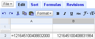
Of course 19! is not 121645100408831984, but 121645100408832000, off by 16. The puzzlement continued when I wrote:

Though the values at B2 and B3 are displayed differently, they compare the same. What's going on here? Actually, B3 is not holding a number but the string "121645100408832000", hence its left alignment --numbers are displayed right-aligned by default. Once we force "121645100408832000" to be internally translated to a number the glitch reappears; it suffices to enter the value as "=121645100408832000":

After thinking a bit about it I realized the value 19! has 57 binary digits, and this rang a bell: if values were stored in double precision IEEE 754 format, with fraction width of 52 bits, not all integers greater than 253 would have exact representation, and in fact 253 + 1 would be the first non-representable integer:

The figure above seems to confirm the hypothesis. For 224 +1 the representation is exact, which seems to rule out single precision IEEE 754 with its 23 bit fraction. In fact, I tested all the values 2n + 1 for n = 1,...,54, and the representation is exact except for n = 54. Further confirmation of the double precision IEEE 754 hypothesis comes from the following:

Does this explain it all? Well, not entirely. The binary representation of 19! is

110110000001010111001001100000110100010010000000000000000.

Thanks to the 16 trailing zeros, this is exactly representable in double precision IEEE 754 as:

19! = s·2e − 1023·1.f,
s = 0,
e = 100001101112 = 1079 = 56 + 1023,
f = 10110000001010111001001100000110100010010000000000002.

So there must be additional problems apart from the loss of precision due to the use of floating point. We will investigate the issue further in a later entry.